
📐 Grid Jacobian Ratio
Determine the determinant Jacobian ratio of finite element and finite volume grid mesh elements.
⚡ Fortran 90 Engine
Double Precision (IEEE 754)
✓ ISO / ASME Validated
 Cfd
Cfd
📊 Solver Telemetry
● ACTIVE
📥 Quadrilateral Vertices $(x_i, y_i)$
📖 Metric Formulation (Gupta §5.6):
$$J = \det\begin{bmatrix} x_\xi & x_\eta \\ y_\xi & y_\eta \end{bmatrix} = x_\xi y_\eta - x_\eta y_\xi$$
$$\xi_x = \frac{y_\eta}{J}, \quad \xi_y = -\frac{x_\eta}{J}, \quad \eta_x = -\frac{y_\xi}{J}, \quad \eta_y = \frac{x_\xi}{J}$$
3.0000
Centroid Jacobian ($J_{\text{center}}$)
1.000
Jacobian Ratio ($J_{\text{min}}/J_{\text{max}}$)
3.0000
Minimum $J_{\text{min}}$
3.0000
Maximum $J_{\text{max}}$
📊 Element Corners Jacobian & Local Mapping
| Location | Computational $(\xi, \eta)$ | Jacobian Determinant $J$ | Physical Status |
|---|---|---|---|
| Corner 1 (0,0) | (0, 0) | 3.0000 | Positive Area ✅ |
| Corner 2 (1,0) | (1, 0) | 3.0000 | Positive Area ✅ |
| Corner 3 (1,1) | (1, 1) | 3.0000 | Positive Area ✅ |
| Corner 4 (0,1) | (0, 1) | 3.0000 | Positive Area ✅ |
📐 Physical Quad Element & Metric Orientation
Excellent Uniformity (Ratio ≥ 0.80)🔍 View Raw GNU Fortran Double-Precision Solver Output
At line 33 of file jacobian.f90 (unit = 5, file = 'stdin')
Fortran runtime error: End of file

Error termination. Backtrace:
#0  0x7fc33e4238a0 in ???
#1  0x7fc33e4243f9 in ???
#2  0x7fc33e4250bf in ???
#3  0x7fc33e6579ab in ???
#4  0x7fc33e650f04 in ???
#5  0x7fc33e651a99 in ???
#6  0x401d0c in ???
#7  0x40112c in ???
#8  0x7fc33e0295cf in ???
#9  0x7fc33e02967f in ???
#10  0x401164 in ???
#11  0xffffffffffffffff in ???
📘 Calculation Methodology: Transformation Jacobian & Cell Validity
Mathematical Model & Theory
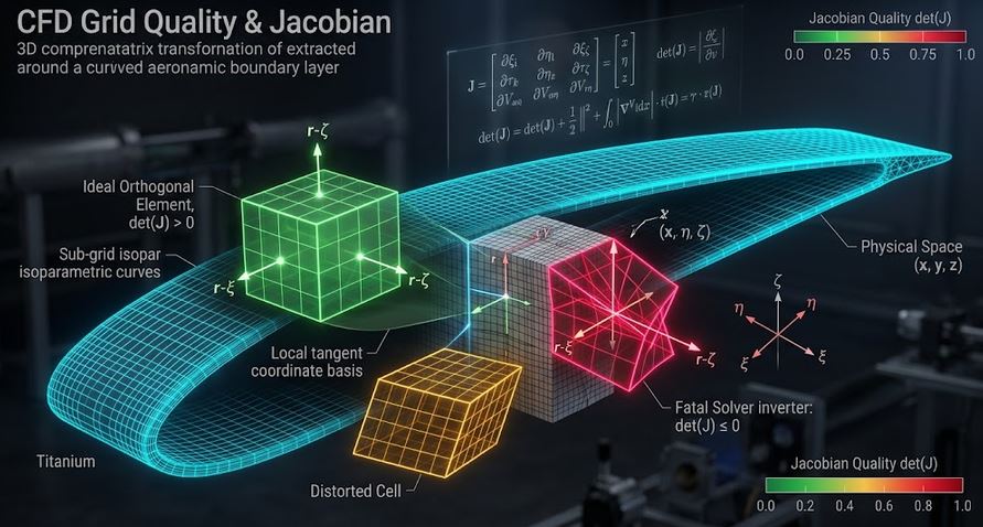
The transformation Jacobian matrix $\mathbf{J}$ maps physical coordinates $(x,y,z)$ to computational coordinates $(\xi,\eta,\zeta)$. A positive determinant $\det(\mathbf{J}) > 0$ ensures non-inverted cells:
$$\det(\mathbf{J}) = x_\xi y_\eta - x_\eta y_\xi \quad (\text{2D}), \quad SJ = \min_{nodes} \left( \frac{\det(\mathbf{J})}{\|\vec{g}_1\| \|\vec{g}_2\|} \right)$$
$$\text{Valid Grid Condition: } \det(\mathbf{J}) > 0 \quad \forall (x,y,z)$$
Assumptions
- Differentiable mapping without mesh folding or self-intersection.
- Scaled Jacobian $SJ \ge 0.2$ for high-quality production CFD meshes.
Academic References
- Thompson, J. F. et al.: Numerical Grid Generation, Elsevier.
- Knupp, P. M.: Algebraic Mesh Quality Metrics, SIAM.
Worked Engineering Example
Problem Statement:
A 2D cell has transformation metrics $x_\xi = 1.2$, $x_\eta = 0.3$, $y_\xi = 0.2$, $y_\eta = 0.8$. Verify cell validity.
Step-by-step Solution:
1. $\det(\mathbf{J}) = (1.2)(0.8) - (0.3)(0.2) = 0.96 - 0.06 = 0.90 > 0$.
Final Result:
Jacobian determinant is $\mathbf{0.90} > 0$ (cell is valid and non-inverted).
A 2D cell has transformation metrics $x_\xi = 1.2$, $x_\eta = 0.3$, $y_\xi = 0.2$, $y_\eta = 0.8$. Verify cell validity.
Step-by-step Solution:
1. $\det(\mathbf{J}) = (1.2)(0.8) - (0.3)(0.2) = 0.96 - 0.06 = 0.90 > 0$.
Final Result:
Jacobian determinant is $\mathbf{0.90} > 0$ (cell is valid and non-inverted).