
🚰 Pump & System Curve Calculator
Solve centrifugal pump operating points for single, parallel, or series configurations. Model pipeline resistance, Colebrook friction losses, and check NPSH cavitation safety.
⚡ Fortran 90 Engine
Double Precision (IEEE 754)
✓ ISO / ASME Validated
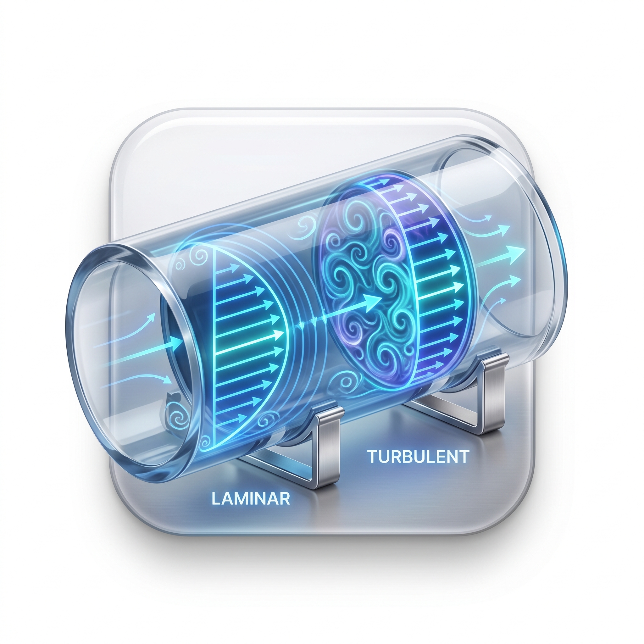 Fluid Mechanics
📊 Solver Telemetry
● ACTIVE
👁️ Views
911
⚡ Solves
713
💾 Downloads
514
📦 Fortran Code
4.5 KB
📅 Released
Jun 2026
⏱️ Latency
< 1 ms
💡
Hardware & Sizing Partner: Need to size a control valve or check ASME flange bolt torque for this line?
📝 Configuration
📊 System Curves & Results
📊 Results Summary
Operating Flow Rate ($Q_{op}$)
110.00 m³/h
30.56 L/s
Operating Head ($H_{op}$)
18.45 m
180.93 kPa
Pump Efficiency ($\eta$)
74.5 %
Peak: 75.0 %
Required Shaft Power
7.43 kW
9.96 HP
NPSH Available ($\text{NPSHa}$)
10.52 m
Required: 3.00 m
Cavitation Check
🟢 SAFE
Margin: 7.52 m
Total Operating Flow ($Q_{op,tot}$)
142.03 m³/h
Per pump: 71.01 m³/h
Operating Head ($H_{op}$)
23.93 m
234.65 kPa
Individual Pump Eff.
62.5 %
Operating point load
Total Shaft Power (2 Pumps)
14.82 kW
Each: 7.41 kW
NPSH Available ($\text{NPSHa}$)
11.43 m
Based on $Q_{total}/2$
Cavitation Check
🟢 SAFE
Margin: 8.43 m
Operating Flow Rate ($Q_{op}$)
144.95 m³/h
40.26 L/s
Total System Head ($H_{op,tot}$)
24.49 m
Per pump: 12.25 m
Individual Pump Eff.
71.8 %
Operating point load
Total Shaft Power (2 Pumps)
13.48 kW
Each: 6.74 kW
NPSH Available ($\text{NPSHa}$)
9.37 m
First stage inlet
Cavitation Check
🟢 SAFE
Margin: 6.37 m
📉 System Runout Flow: 139.10 m³/h (Maximum possible system discharge capacity at zero static head differential).
📈 System Curve Equation: $H_{sys}(Q) = 10.0 + K_{fric}(Q) \cdot Q^2$
📈 System Curve Equation: $H_{sys}(Q) = 10.0 + K_{fric}(Q) \cdot Q^2$
📈 Pump Curve & System Resistance Curve Overlay (Q in m³/h vs Head in m)
Single Pump
Parallel Curve
Series Curve
System Curve
Efficiency [%]
🖨️ Raw Fortran Output
Pump A =      -0.000500
Pump B =      -0.050000
Pump C =      30.000000
Single Q =       110.0034
Single H =        18.4495
Single Eff =          74.48
Single Power =         7.4254
Single NPSHa =        10.5186
Parallel Q =       142.0298
Parallel H =        23.9277
Parallel Eff =          62.50
Parallel Power =        14.8167
Parallel NPSHa =        11.4299
Series Q =       144.9498
Series H =        24.4946
Series Eff =          71.76
Series Power =        13.4829
Series NPSHa =         9.3720
Runout Flow =       139.1010
📘 Calculation Methodology
Mathematical Model & Theory
A centrifugal pump operates at the intersection of its head-capacity performance curve ($H_{pump}$) and the pipeline network's system resistance curve ($H_{sys}$):
$$H_{sys}(Q) = \Delta z + h_f + h_m = \Delta z + \left( f\frac{L}{D} + \sum K \right) \frac{V^2}{2g}$$
The Darcy friction factor $f$ is solved dynamically for the active Reynolds number ($\text{Re} = \rho V D / \mu$) using the implicit **Colebrook-White equation** solved via successive approximations:
$$\frac{1}{\sqrt{f}} = -2.0 \log_{10}\left( \frac{\epsilon}{3.7 D} + \frac{2.51}{\text{Re}\sqrt{f}} \right)$$
For dual pump configurations, combined curves are constructed:
- Parallel Configuration: Double the capacity at a given head ($Q_{tot} = 2 \cdot Q_{single}$). Suitable for high flow rates and flat system curves.
- Series Configuration: Double the head at a given capacity ($H_{tot} = 2 \cdot H_{single}$). Suitable for high static heads and steep system curves.
Academic References
- Karassik, Igor J.: Pump Handbook, McGraw-Hill.
- Hydraulic Institute: Centrifugal Pumps: Design and Application.
- Cengel, Y. & Cimbala, J.: Fluid Mechanics: Fundamentals and Applications, McGraw-Hill.
Worked Engineering Example
Problem Statement:
A piping system requires lifting water ($\rho = 1000\text{ kg/m³}, \mu = 0.001\text{ Pa·s}$) by $\Delta z = 10\text{ m}$ through a $D = 100\text{ mm}$ pipe of length $L = 50\text{ m}$ ($\epsilon = 0.05\text{ mm}, \Sigma K = 2.0$). The pump curve is given by the Medium Head preset: $H_p(Q) = 30.0 - 0.05Q - 0.0005Q^2$ ($Q$ in $\text{m³/h}$). Find the operating point for a single pump.
Step-by-step Solution:
1. System Curve expression for flow rate $Q$:
$$V = \frac{Q\text{ [m³/h]}}{3600 \cdot \frac{\pi}{4} D^2} = 0.03537 \cdot Q\text{ m/s}$$ For $Q = 110\text{ m³/h}$, $V \approx 3.89\text{ m/s}$, giving $\text{Re} \approx 3.89 \times 10^5$.
Solving Colebrook's equation gives $f \approx 0.0177$.
2. Calculate total system head at $Q = 110\text{ m³/h}$:
$$h_{loss} = \left( 0.0177 \frac{50}{0.1} + 2.0 \right) \frac{3.89^2}{2 \times 9.81} \approx 8.45\text{ m}$$ $$H_{sys} = 10.0 + 8.45 = 18.45\text{ m}$$ 3. Evaluate pump head at $Q = 110\text{ m³/h}$:
$$H_p = 30.0 - 0.05(110) - 0.0005(110)^2 = 30.0 - 5.5 - 6.05 = 18.45\text{ m}$$ 4. Since $H_{pump}(110) = H_{sys}(110) = 18.45\text{ m}$, the operating point is at:
$$Q_{op} = 110.0\text{ m³/h}, \quad H_{op} = 18.45\text{ m}$$
A piping system requires lifting water ($\rho = 1000\text{ kg/m³}, \mu = 0.001\text{ Pa·s}$) by $\Delta z = 10\text{ m}$ through a $D = 100\text{ mm}$ pipe of length $L = 50\text{ m}$ ($\epsilon = 0.05\text{ mm}, \Sigma K = 2.0$). The pump curve is given by the Medium Head preset: $H_p(Q) = 30.0 - 0.05Q - 0.0005Q^2$ ($Q$ in $\text{m³/h}$). Find the operating point for a single pump.
Step-by-step Solution:
1. System Curve expression for flow rate $Q$:
$$V = \frac{Q\text{ [m³/h]}}{3600 \cdot \frac{\pi}{4} D^2} = 0.03537 \cdot Q\text{ m/s}$$ For $Q = 110\text{ m³/h}$, $V \approx 3.89\text{ m/s}$, giving $\text{Re} \approx 3.89 \times 10^5$.
Solving Colebrook's equation gives $f \approx 0.0177$.
2. Calculate total system head at $Q = 110\text{ m³/h}$:
$$h_{loss} = \left( 0.0177 \frac{50}{0.1} + 2.0 \right) \frac{3.89^2}{2 \times 9.81} \approx 8.45\text{ m}$$ $$H_{sys} = 10.0 + 8.45 = 18.45\text{ m}$$ 3. Evaluate pump head at $Q = 110\text{ m³/h}$:
$$H_p = 30.0 - 0.05(110) - 0.0005(110)^2 = 30.0 - 5.5 - 6.05 = 18.45\text{ m}$$ 4. Since $H_{pump}(110) = H_{sys}(110) = 18.45\text{ m}$, the operating point is at:
$$Q_{op} = 110.0\text{ m³/h}, \quad H_{op} = 18.45\text{ m}$$