
📐 Supersonic Conical Shock (Taylor-Maccoll)
Solve 3D axisymmetric supersonic conical flow, computing attached conical shock wave angle (θs), cone surface Mach (Mc), surface pressure coefficient (Cp), and wave drag (CDw).
⚡ Fortran 90 Engine
Double Precision (IEEE 754)
✓ ISO / ASME Validated
 Cfd
Cfd
📊 Solver Telemetry
● ACTIVE
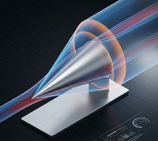
📐 Supersonic Axisymmetric Cone & Attached Conical Shock Wave
Real-time visual simulation of 3D conical flow streamlines deflecting across Taylor-Maccoll shock cone📝 Configuration & Presets
🚀 Missile Cone (Mach 2.5, 15°)
🎯 Interceptor (Mach 4.0, 20°)
⚡ Hypersonic Sharp (Mach 6, 10°)
✈️ Pitot Probe (Mach 1.8, 12°)
Taylor-Maccoll Conical Formulations:
• Conical Shock Angle: θs < βwedge (3D relief effect)
• Surface Pressure Coeff: Cp = (Pc − P₁) / (½ γ P₁ M₁²)
• Conical Wave Drag: CD,wave = Cp (referenced to base area)
• Shock Jump: P₂/P₁ = [ 2γ (M₁ sin θs)² − (γ−1) ] / (γ+1)
• Conical Shock Angle: θs < βwedge (3D relief effect)
• Surface Pressure Coeff: Cp = (Pc − P₁) / (½ γ P₁ M₁²)
• Conical Wave Drag: CD,wave = Cp (referenced to base area)
• Shock Jump: P₂/P₁ = [ 2γ (M₁ sin θs)² − (γ−1) ] / (γ+1)
📊 Conical Aerodynamic Results
Configure inputs and click Compute to view results.
📘 Calculation Methodology & Taylor-Maccoll Standards
3D Axisymmetric Conical Relief
Unlike a 2D planar wedge where flow behind the shock is uniform, flow past a cone undergoes continuous isentropic 3D expansion between the shock and cone surface:
θs,cone < βwedge & Pcone < Pwedge
Taylor-Maccoll Differential Solution
Ray velocity $V_r(\theta)$ and tangential velocity $V_\theta(\theta)$ obey the non-linear ODE subject to tangency $V_\theta(\theta_c) = 0$ at the cone wall.
Key Engineering Assumptions
- Attached conical shock wave ($M_1 > 1.1$, $\theta_c < \theta_{c,max}$).
- Calorically perfect inviscid gas ($\gamma = 1.40$).
- Zero angle of attack ($\alpha = 0^\circ$ axisymmetric alignment).