🏙️ Atmospheric Boundary Layer Wind Profile

Calculate atmospheric boundary layer wind velocity gradient using Log-Law and Power-Law, dynamic wind stagnation pressure on facades, and base overturning moments.

⚡ Fortran 90 Engine Double Precision (IEEE 754) ✓ ISO / ASME Validated

Cfd

📊 Solver Telemetry ● ACTIVE

👁️ Views 15

⚡ Solves 13

💾 Downloads 511 📦 Fortran Code 4.4 KB

📅 Released Jun 2026

⏱️ Latency < 1 ms

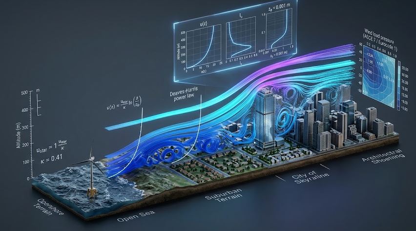
🏙️ Atmospheric Boundary Layer & Vertical Wind Velocity Gradient

Real-time visual simulation of ground roughness shear, logarithmic velocity profile & high-rise structural drag

📝 Configuration & Presets

🏙️ City Skyscraper (200m) 🌊 Offshore Wind Mast (140m) 🏭 Suburban Warehouse 📡 Rural Mast (100m)

💨 Reference Wind & Terrain

Reference Wind Speed U_ref [m/s]: Standard at 10m height (e.g. 25 m/s ≈ 90 km/h)

Terrain Roughness Length z₀ [m]: Sea: 0.002, Open: 0.03, Suburb: 0.30, City: 1.0–2.0

Power-Law Exponent α: Sea: 0.12, Open: 0.16, City: 0.33

Air Density ρ [kg/m³]:

🏢 Building / Structure Dimensions

Building Height H [m]:

Facade Width W [m]:

ABL Wind Engineering Formulations:
• Log-Law Profile: U(z) = (u*/κ) · ln(z / z₀) [m/s]
• Friction Velocity: u* = (κ · U_ref) / ln(z_ref / z₀)
• Dynamic Stagnation Pressure: q(z) = ½ ρ [U(z)]² [Pa]
• Turbulence Intensity: I_z(z) ≈ 1 / ln(z / z₀)

📊 Wind Engineering Results

Configure inputs and click Compute to view results.

📘 Calculation Methodology & ASCE 7 / Eurocode 1 Standards

Atmospheric Logarithmic Law

Derived from Prandtl mixing length theory for neutral atmospheric boundary layer equilibrium over rough terrain:

                    U(z) = (u* / κ) · ln(z / z₀)
                

Dynamic Wind Pressure & Overturning

Dynamic wind stagnation pressure scales quadratically with height: $q(z) = \frac{1}{2} \rho [U(z)]^2$, creating substantial overturning moments on high-rise structures.

Key Engineering Assumptions

Neutral atmospheric thermal stability (no strong convective inversions).
Homogeneous fetch and uniform aerodynamic terrain roughness $z_0$.
von Kármán constant $\kappa = 0.40$.

ThermoFluidCalc Engineering Report